symbols

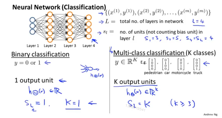
L ：神经网络的层数

S_l ：第 l 层神经网络的神经元数

K ：分类个数

10神经网络分类问题

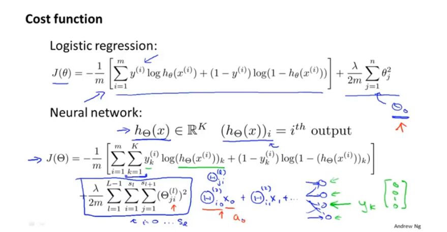
代价函数

从逻辑回归算法中衍生到神经网络

每个 logistic regression algorithm 的代价函数然后 K次输出最后求和。

不对偏置单元(bias)进行正则化操作，即含X_0的项

10神经网络分类问题-代价函数

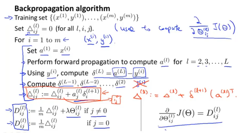
步骤

定义：误差项 delta(l)_j 表示第 l 层的第 j 的激活值与y之间的误差。

10神经网络分类问题-误差项

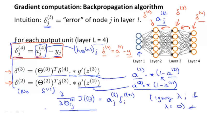
不严谨地说：在忽略lambda(正则项)或lambda=0，误差项 = 相应的代价项的偏导由此可以计算出所需参数。

综上：

▲是大写的delta

10神经网络反向传播步骤

更好地理解

delta(l)_j 其实是代价函数关于Z(l)__j的偏导，其值只计算隐藏单元而不计算偏置单元。

10神经网络分类问题-误差项

参数

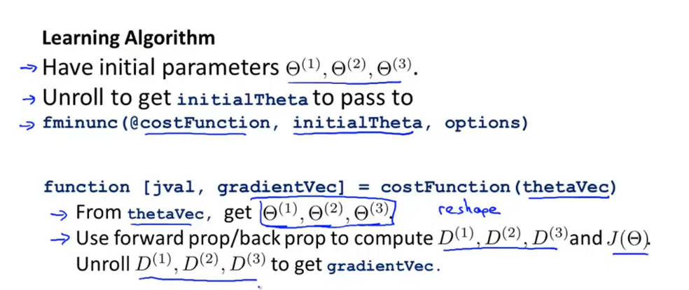
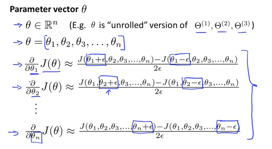
矩阵与向量

公式中参数的形式均为向量，所以需要将矩阵转化为向量形式。

矩阵->向量： a = [ b1(:); b2(:); b3(:) ]

向量->矩阵： b1 = reshape(a(1:110),10,11); %向量前110个数组成10行11列的矩阵。

10神经网络分类问题-参数

梯度检测

（1）梯度估计

10神经网络分类问题-梯度估计

（2）J(θ)偏导数

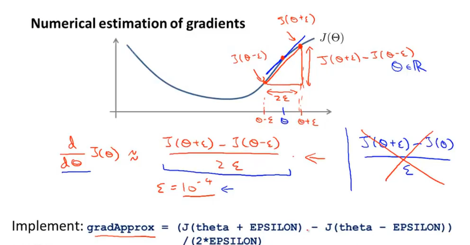
10神经网络分类问题-θ偏导数

（3）检查J(θ)偏导数是否等于反向传播的导数，近似相等则反向传播正确实现

10神经网络分类问题-θ偏导数代码

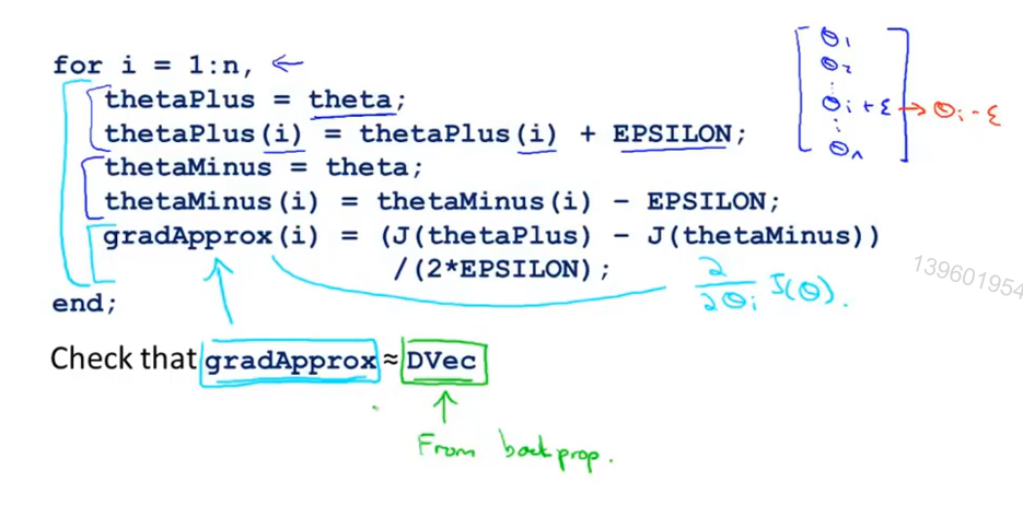
综合检测步骤：

注意在正确之后，关闭梯度检测再进行训练分类器。

10神经网络分类问题-θ偏导数代码

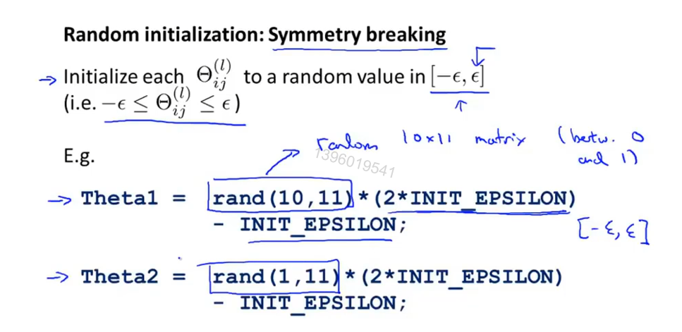
θ随机初始化

防止 θ值相同，限制学习模型的特征输入

10神经网络分类问题-θ随机初始化

总结

训练神经网络

（1）选择网络架构：输入特征项数，输出分类项，隐藏层（1个或者多个但每层隐藏单元相同）

（2）随机初始化θ

（3）完成前向传播算法得到h_θ(x)

（4）完成代价函数 J(θ) 的计算

(5) 完成反向传播算法得到 J关于θ的偏导数

（6）遍历训练集，运行前向传播算法和反向传播算法，得到每层激活项a(l)与delta(l)

（7）梯度检查

（8）高级优化算法与反向传播算法结合计算min J.

编程作业

nnCostFunction.m

function [J grad] = nnCostFunction(nn_params, ...
                                   input_layer_size, ...
                                   hidden_layer_size, ...
                                   num_labels, ...
                                   X, y, lambda)
%NNCOSTFUNCTION Implements the neural network cost function for a two layer
%neural network which performs classification
%   [J grad] = NNCOSTFUNCTON(nn_params, hidden_layer_size, num_labels, ...
%   X, y, lambda) computes the cost and gradient of the neural network. The
%   parameters for the neural network are "unrolled" into the vector
%   nn_params and need to be converted back into the weight matrices. 
% 
%   The returned parameter grad should be a "unrolled" vector of the
%   partial derivatives of the neural network.
%

% Reshape nn_params back into the parameters Theta1 and Theta2, the weight matrices
% for our 2 layer neural network
Theta1 = reshape(nn_params(1:hidden_layer_size * (input_layer_size + 1)), ...
                 hidden_layer_size, (input_layer_size + 1));

Theta2 = reshape(nn_params((1 + (hidden_layer_size * (input_layer_size + 1))):end), ...
                 num_labels, (hidden_layer_size + 1));

% Setup some useful variables
m = size(X, 1);
         
% You need to return the following variables correctly 
J = 0;
Theta1_grad = zeros(size(Theta1));
Theta2_grad = zeros(size(Theta2));

% ====================== YOUR CODE HERE ======================
% Instructions: You should complete the code by working through the
%               following parts.
%

% Part 1: Feedforward the neural network and return the cost in the
%         variable J. After implementing Part 1, you can verify that your
%         cost function computation is correct by verifying the cost
%         computed in ex4.m
%将y扩展为5000*10的0/1表示形式
expend = eye(num_labels);
%disp(expend);
disp("\n");
%disp(y(500:505,:));
disp("\n");
y = expend(y,:);
%disp(y(500:505,:));

one = ones(m,1);
a1 = [one,X];
z2 =  Theta1 * a1' ;
a2 = sigmoid(z2);
a2 = [one,a2'];
z3 = a2 * Theta2';
h =  sigmoid(z3);
J = sum(sum((y-1).*log(1-h) - y.*log(h))) / m ;
reg = lambda/2/m * (sum(sum(Theta1(:,2:end).^2)) + sum(sum(Theta2(:,2:end).^2)));
%reg = lambda/2/m *(sum(sum(Theta1.^2)) + sum(sum(Theta2.^2))
%      - sum(sum(Theta1(:,1).^2)) + sum(sum(Theta2(:,1).^2)));
J = J + reg;

%
% Part 2: Implement the backpropagation algorithm to compute the gradients
%         Theta1_grad and Theta2_grad. You should return the partial derivatives of
%         the cost function with respect to Theta1 and Theta2 in Theta1_grad and
%         Theta2_grad, respectively. After implementing Part 2, you can check
%         that your implementation is correct by running checkNNGradients
%
%         Note: The vector y passed into the function is a vector of labels
%               containing values from 1..K. You need to map this vector into a 
%               binary vector of 1's and 0's to be used with the neural network
%               cost function.
%
%         Hint: We recommend implementing backpropagation using a for-loop
%               over the training examples if you are implementing it for the 
%               first time.


delta3 = h - y;
delta2 = delta3 * Theta2 ;
delta2 = delta2(:,2:end);
delta2 = delta2 .* sigmoidGradient(z2)';

D1 = zeros(size(Theta1));
D2 = zeros(size(Theta2));
D1 = D1 + delta2' * a1;
D2 = D2 + delta3' * a2;


%
% Part 3: Implement regularization with the cost function and gradients.
%
%         Hint: You can implement this around the code for
%               backpropagation. That is, you can compute the gradients for
%               the regularization separately and then add them to Theta1_grad
%               and Theta2_grad from Part 2.
%


Theta1_grad = ( D1  + lambda * Theta1 ) / m;
Theta2_grad = ( D2  + lambda * Theta2 ) / m;
Theta1_grad(:,1) = Theta1_grad(:,1) - lambda / m  * Theta1(:,1);
Theta2_grad(:,1) = Theta2_grad(:,1) - lambda / m  * Theta2(:,1);

%找到每个X最大的估计数字，h归一化
% maxValue = max(h,[],2);
% h = (h >= maxValue);



% -------------------------------------------------------------

% =========================================================================

% Unroll gradients
grad = [Theta1_grad(:) ; Theta2_grad(:)];


end

sigmoidGradient.m

function g = sigmoidGradient(z)
%SIGMOIDGRADIENT returns the gradient of the sigmoid function
%evaluated at z
%   g = SIGMOIDGRADIENT(z) computes the gradient of the sigmoid function
%   evaluated at z. This should work regardless if z is a matrix or a
%   vector. In particular, if z is a vector or matrix, you should return
%   the gradient for each element.

g = zeros(size(z));

% ====================== YOUR CODE HERE ======================
% Instructions: Compute the gradient of the sigmoid function evaluated at
%               each value of z (z can be a matrix, vector or scalar).

g = sigmoid(z) .* (1-sigmoid(z));


% =============================================================

end

randInitializeWeights.m

function W = randInitializeWeights(L_in, L_out)
%RANDINITIALIZEWEIGHTS Randomly initialize the weights of a layer with L_in
%incoming connections and L_out outgoing connections
%   W = RANDINITIALIZEWEIGHTS(L_in, L_out) randomly initializes the weights 
%   of a layer with L_in incoming connections and L_out outgoing 
%   connections. 
%
%   Note that W should be set to a matrix of size(L_out, 1 + L_in) as
%   the first column of W handles the "bias" terms
%

% You need to return the following variables correctly 
W = zeros(L_out, 1 + L_in);

% ====================== YOUR CODE HERE ======================
% Instructions: Initialize W randomly so that we break the symmetry while
%               training the neural network.
%
% Note: The first column of W corresponds to the parameters for the bias unit
%

epsilon_init = 0.12;
W = rand(L_out, 1 + L_in)*2*epsilon_init  - epsilon_init;



% =========================================================================

end