机器学习-逻辑回归

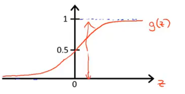
sigmoid function also logistic function

“分类问题”–逻辑回归算法

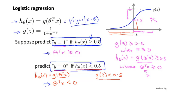
决策边界 不是训练集的属性，而是假设本身和其参数的属性

计算的是 属于1 的概率

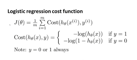
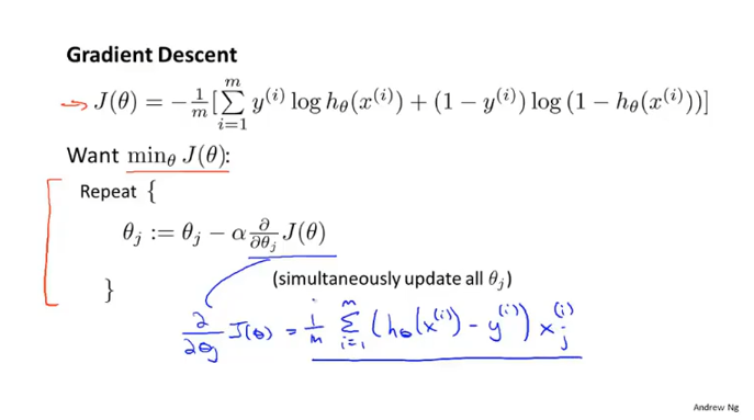
cost function

适用于梯度下降的变形式：

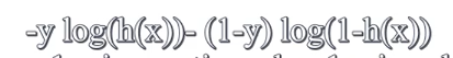
综上：

来源于统计学的极大似然估计法—-凸函数

高级优化

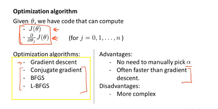
使用库~直接调用，适用于大型的机器学习

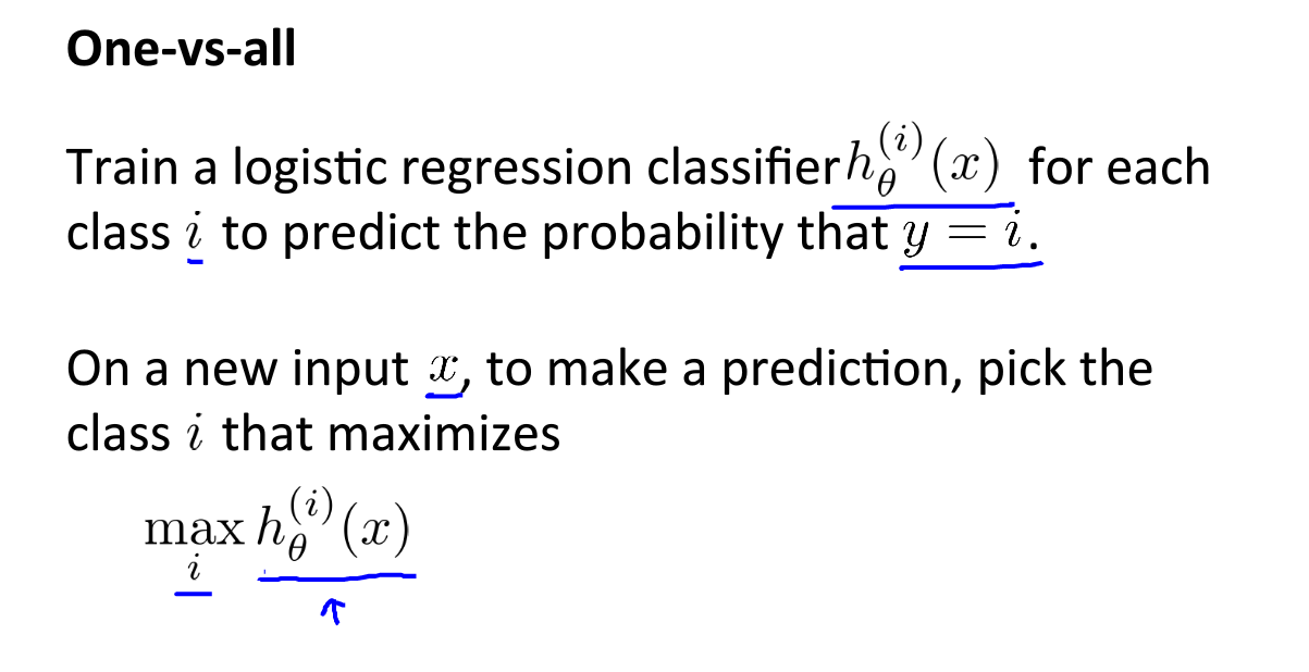
多元分类：”一对多“分类

采用多个分类器，针对其中一种情况进行训练

拟合

泛化 ：一个假设模型应用到新样本的能力~

欠拟合/过拟合 高方差

减少特征变量

但是同时舍弃了一些有用信息

正则化

简化假设模型，更少的倾向过拟合

线性回归正则化

后一项是正则化项

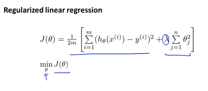
不惩罚 θ_0

（1）梯度下降：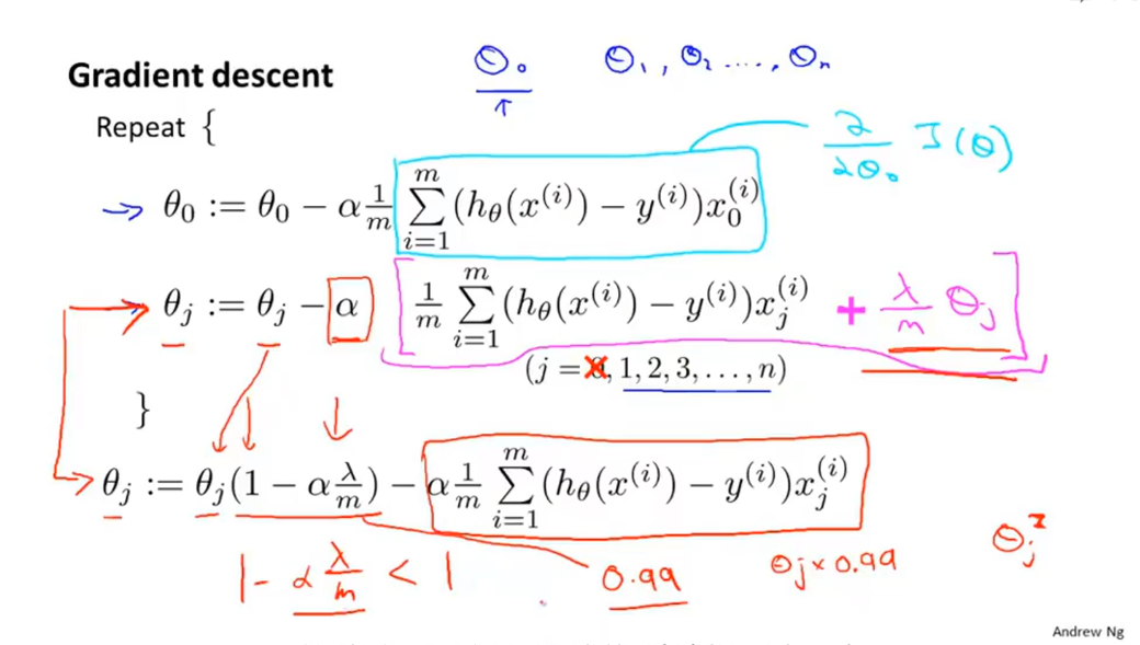

（2）正则化方程：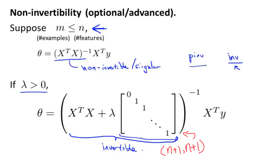

虽然octave在一般的正则化方程中 pinv() 可能会给 奇异矩阵 可逆结果，但是这不能泛化。但经过正则化 正则方程后，一定是可逆的。

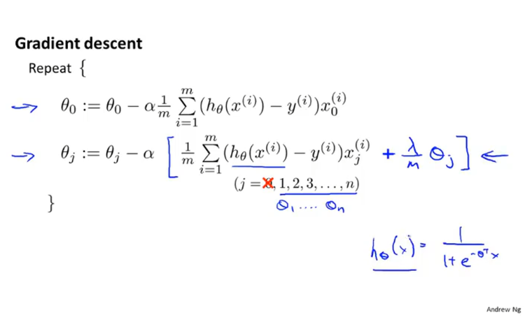
逻辑回归正则化

不惩罚 θ_0

注意：虽然看起来和 线性回归一样，但是 h(x)不同

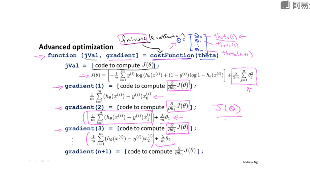
（3）高级算法：

fminunc() :函数在无约束条件下的最小值

不需要写任何循环，也无需设置循环；只需要提供一个计算“代价”和“梯度”的函数，就返回正确的优化参数、代价值、θ

tips: octave下标从1开始。。

编程作业

costFunction.m

function [J, grad] = costFunction(theta, X, y)
%COSTFUNCTION Compute cost and gradient for logistic regression
%   J = COSTFUNCTION(theta, X, y) computes the cost of using theta as the
%   parameter for logistic regression and the gradient of the cost
%   w.r.t. to the parameters.

% Initialize some useful values
m = length(y); % number of training examples

% You need to return the following variables correctly 
J = 0;
grad = zeros(size(theta));

% ====================== YOUR CODE HERE ======================
% Instructions: Compute the cost of a particular choice of theta.
%               You should set J to the cost.
%               Compute the partial derivatives and set grad to the partial
%               derivatives of the cost w.r.t. each parameter in theta
%
% Note: grad should have the same dimensions as theta
%


h = sigmoid(X * theta);
J = sum( log(1-h)'*(y-1) - log(h)'*y )/m;
grad = X' * (h - y)/m;

% =============================================================

end

costFunctionReg.m

function [J, grad] = costFunctionReg(theta, X, y, lambda)
%COSTFUNCTIONREG Compute cost and gradient for logistic regression with regularization
%   J = COSTFUNCTIONREG(theta, X, y, lambda) computes the cost of using
%   theta as the parameter for regularized logistic regression and the
%   gradient of the cost w.r.t. to the parameters. 

% Initialize some useful values
m = length(y); % number of training examples

% You need to return the following variables correctly 
J = 0;
grad = zeros(size(theta));

% ====================== YOUR CODE HERE ======================
% Instructions: Compute the cost of a particular choice of theta.
%               You should set J to the cost.
%               Compute the partial derivatives and set grad to the partial
%               derivatives of the cost w.r.t. each parameter in theta

h = sigmoid(X * theta);
J = sum( log(1-h)'*(y-1) - log(h)'*y )/m + lambda/2/m  * (sum(theta.^2)- theta(1)^2);

for j = 1:length(theta)
  if j == 1
  grad(j)=  ((h - y)' * X(:,j)) /m;
  else
  grad(j) = ( (h - y)' * X(:,j) + theta(j)*lambda) / m; 
end

%另一种方法：
%grad = X' * (h - y)/m + theta*lambda / m; 
%grad(1) = grad(1) -theta(1)*lambda / m;

% =============================================================

end

plotData.m

function plotData(X, y)
%PLOTDATA Plots the data points X and y into a new figure 
%   PLOTDATA(x,y) plots the data points with + for the positive examples
%   and o for the negative examples. X is assumed to be a Mx2 matrix.

% Create New Figure
figure; hold on;

% ====================== YOUR CODE HERE ======================
% Instructions: Plot the positive and negative examples on a
%               2D plot, using the option 'k+' for the positive
%               examples and 'ko' for the negative examples.
%

%pos = find(y == 1);
neg = find(y == 0);

%plot(X(pos,1), X(pos,2), 'k+', 'LineWidth', 2, 'MarkerSize', 7);
plot(X(neg,1),X(neg,2), 'ko', 'markerFaceColor', 'y', 'MarkerSize', 7);

% =========================================================================
hold off;

end

predict.m

function p = predict(theta, X)
%PREDICT Predict whether the label is 0 or 1 using learned logistic 
%regression parameters theta
%   p = PREDICT(theta, X) computes the predictions for X using a 
%   threshold at 0.5 (i.e., if sigmoid(theta'*x) >= 0.5, predict 1)

m = size(X, 1); % Number of training examples

% You need to return the following variables correctly
p = zeros(m, 1);

% ====================== YOUR CODE HERE ======================
% Instructions: Complete the following code to make predictions using
%               your learned logistic regression parameters. 
%               You should set p to a vector of 0's and 1's
%

p = sigmoid(X * theta);
rows = size(p,1);
cols = size(p,2);
for i = 1:rows
   for j = 1:cols
    
	if p(i,j) < 0.5
      p(i,j) = 0;
	else
	  p(i,j) = 1;
   end
end


%p = sigmoid(X*theta)>0.5;
% =========================================================================


end

sigmoid.m

function g = sigmoid(z)
%SIGMOID Compute sigmoid function
%   g = SIGMOID(z) computes the sigmoid of z.

% You need to return the following variables correctly 
g = zeros(size(z));

% ====================== YOUR CODE HERE ======================
% Instructions: Compute the sigmoid of each value of z (z can be a matrix,
%               vector or scalar).
%rows = size(z)(1);
%cols = size(z)(2);
%if rows == 1 && cols == 1

    one = ones(size(z));
	g = one ./ (1 + exp(-z));

% =============================================================

end